Self-supervised learning methods
A clever tale of augmentations
What is self-supervised learning ?
Self supervised learning aims to train a machine learning model, without having access to any labelled data. Un-supervised learning is the class of models which don’t require training labels.
What is so special about it then? Has not unsupervised learning existed for decades already now?
No. Even though unsupervised models aka Clustering have existed for sometime now, they have not utilitzed much progress already made in Deep learning.
In my opinion ,what distinguishes recent self supervised learning is the clever way in which these approaches change an unlabeled dataset, to a pseudo labeled dataset . Often times , these models also make user of “contrastive loss” objectives to train .
What do I mean by a pseudo labeled dataset ? Read through this blog to find out more ……….
First questions first : Why is this interesting ?
Usually academics, companies and institutions have a lot more of unlabled data available than the amount of labelled data.
The progress in Supervised learning has been impressive, but it has been dependent on “labelled data”. Good quality annotations and labels are always needed. Model training is sensitive to noisy labels, and quality checks restrict scaling of dataset size. In fact data labelling can be a very laborious (and expensive ) process and has actually given birth to some companies solving for this problem , Amazon Mechanical Turks or Playment.
But you don’t want to spend so much . Not because you are cheap. But because there has to be a better way .
Enter Self-supervised learning…., and now Unsupervised learning is cool again.
What is a Contrastive loss ?
Contrastive loss is at the heart of this Self Supervised paradigm. A contrastive loss uses a distance measure between positive samples and negative samples to train a model.
It attempts to decrease the loss (think distance) value between two very similar samples, while simultaneously increasing the loss value between dissimilar samples.
Surprisingly this technique has been around for sometime. We can retrospectively see that the old model Word2Vec was also a semi-supervised learning model.
If we re-read to the paper by Mikolov et al, we would see a very similar loss :

To train the model, Word2Vec tries to learn the distribution of “neighbouring” words for a “target word”. For example, according to the Skip gram approach, if we have the sentence “this is an old castle”, you could take out the word “old”, and try to predict the nearby words “this ,is, an, castle “. This shall be an instance of positive example. To make model training easier, we can also sample some random words which are not going to fit this sentence, with the belief that these “contrastive” examples teach the model what is a wrong sentence construction.
“Negative samples” are seen as obvious contrasts to your positive sample, which would make it easy for your model to learn a representation which differentiates between “positive samples” (similar examples) or the “negative samples”.
In self supervised approaches instead of doing random sampling , and letting fate take control, our programs take charge. And we create/craft “useful” positive or negative samples through random transformations, which we will henceforth call as augmentations
Augmentations can be simple random operations. For an image sample, you could rotate the image or crop it or flip it or add noise. Or do all of them.
What is the deal with these augmentations?
Ideally we want to “pretrain” our models on large datasets to capture as much “semantic information” as possible on the whole wide world (think internet).
But wait, what does it mean to capture “semantic information”. It means we want our models to capture useful concepts instead of something like a shortcut. Say if you have an image classification task between cats and dogs. Ideally you would want your model to learn that there is a difference between the two animals because of the shape of their snouts, their eyes and their overall sizes.
But as it often happens with high capacity models, your model would cheat , and learn to predict with high accuracy just by memorizing that most cats are either black or white , while dogs are brown . We don’t want this “overfitting” as it compromises the prediction quality.
Hence we would want to force the model, to not learn these non-meaningful things, by adding augmentations to our data.
Creating different augmentations for different data modalities (text, images etc) has been seen as an important future research decision.
SimCLR :
Paper A Simple Framework for Contrastive Learning of Visual Representations Chen et al
The purpose of this framework is to use a contrastive objective to learn a model on huge sets of unlabeled data. We begin with 1 input sample and then do two series(choose any set of suitable augmentations ) of augmentations on it. We as humans know that the two augmented samples, are practically the same thing as flipping an image or rotating it doesn’t semantically change it. But teaching this task to the program would be our training objective. All other remaining samples, which are not “related” to this sample, can be effectively seen as negatives. (Check the batch similarity matrix below if this was not clear to you).
The SimCLR framework involves use of two modules, 1)the encoder and 2) the projection layer.
We train our model on the contrastive loss, till it goes down to model convergence. Once our model has learnt the task, we shall be only using the “encoder” and ditch the projection layer . Interestingly the framework is model agnostic and we can choose any suitable encoder for our task.
According to my understanding the purpose of the projection layer is to output z. “Z” has been brought to a vector dimension $[X]$ (that is a vector shape), so that the dot product similarity can be calculated between $z_1, z_2$ . You can’t calculate similarity values for a matrix $[X x Y]$
Architecture
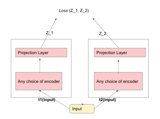
Do remember that for every sample we start with, we end up having 2 of those samples, due to the augmentation. Hence if our original batch size is $K$, the batch size at run time would be $2K$. t1 and t2 are the random augmentation functions .
The loss function here is :
$ \LARGE l_{i,j} = -\log \frac{\exp( \frac{sim(z_i , z_j)}{\tau} )} {\sum_{k=1}^{2N} {\bold{1_{k \neq i}}} \exp( \frac{sim(z_i , z_k)}{\tau} ) } $
Any flashbacks of the Word2Vec loss?
Notice the 2N terms in the denominator sum.
In my implementation I used cosine similarity to capture “similarities”. Cosine simialrity values range between $[-1,1]$
The numerator has similarity between the positive pairs, $i,j$. Positive pairs are the pairs of samples which were synthetically augmented from 1 single sample. The cosine similarity between any of these original $i,j$ positive samples “needs” to go towards $1$ by the end of training.
The denominator captures the cosine similarity between one sample and rest of the non related $2k-2$ samples (remember our batch size at run time is 2K). The cosine similarity between the non-related or “negative samples”, needs to go as low as possible (ideally -1).
$\tau$ is termed as the temperature , which is generally used to control how sharp the output of a Softmax funciton is . By sharpness, I mean that a high temperature value, leads to softmax results which are all close to each other (soft). A very low temperature (say a fractional value :0.2), would lead to sharper differences between the softmax outputs (also called hard).
Example: In a simple implementaion if we begin with two data samples, Cat and Dog. We do augmentations on the Cat sample to get , Cat1 and Cat2 samples. And similarly on the second data sample, augmentation gives Dog1 and Dog2. Starting from 2 samples, we have now 4 samples at run time. The similarity matrix would be of dimensions $4 X 4$. If we observe the similarity matrix after training we could have something like this :

Notice the presence of cosine similarity values 1 between positive pairs and and -1 between the negative samples .
Do remember that Batch size is a very important hyper-parameter for SimCLR. A larger batch size means a pair of positive example vs (a much much bigger set of remaining , non-related, negative samples).
BYOL :
Paper Bootstrap your own latent: A new approach to self-supervised Learning DeepMind
The cool thing about this paper is that Negative samples are not needed at all in this framework. This has led some people to believe that it is easier to train , compared to the SimCLR framework.
Architecture

The online network, tries to predict, output of the target network. In other words, it can be imagined as a regression task for the online network, attempting to predict what is the next output of target network.
There is no presence of an explicit “negative sample” in this scenario, but there have been some research speculations that maybe the “batchNorm” present in the predictor adds implicit negative samples.
The model uses a delayed updates of the weights on the target network. This delay is controlled by decay rate ($\tau$):
$ weight_{trg new } = weight_{trg old} * \tau + (1-\tau) * weight_{new online}$
Strangely, the paper reported best results for decay values from 0.9 to 0.999 .
This approach means target network stores the old weights (moving average weights), and we get new updated weights every time for the online network.
Do notice the dashed line on the Target network, which implies No Gradient Backpropagation on this target network.
Though despite of all the talk about absence of negative samples, there has been some research suggesting that batchNorm in the projection and prediction module could be finding negative samples indirectly .
Ending notes
Interestingly both SimCLR and BYOL are seen as model agnostic and independent of the nature of encoder you want to use.
I must also mention that Yannic Kilcher has an amazing video describing BYOL in detail, and I found it very easy to understand many of the model details.