Basics of Graph representation learning
Reading through the basics and applying for detecting rumour propagation networks
Why Graph representation learning?
Graph representation learning is …. tadaa …deep learning for graphs.
The one key factor behind graph representation learning is:
Don’t tamper with a graph dataset.
The structure of the graph itself has probably precious information. Instead of modifying a graph input to be able to feed to our ML models, we feed the Graph as it is. Graph neural networks aim to work with graph datasets directly as their input.
Our models would aim to learn the node embeddings to attach some meaning to the inputs, and then we can train towards predicting downstream tasks such as a node prediction or missing edge prediction.
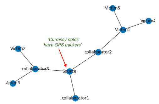
A rumour propagation network with source and collaborator at its heart, spreading rumour outwards to unsuspecting users
For example in this above network, where a source is trying to spread fake news (text), the reshares between collaborators is an easy hint. If our model has understood that the source and collaborators often actively collude together to spreak fake information, it would be easier to red flag fake information, rather than investigating in isolation each share/retweet of the fake content (the original shared rumour text or the fake image in question here).
Outline of this blog
The end goal of this blog would be to learn the ‘theoretical’ working of these three neural networks:
1) GCN (Graph Convolution Network) 2) GAT (Graph Attention Network) 3) Graph Sage
And then apply it to a fake news dataset (UPFD - politifact). I have not written any new code and mostly just borrowed an example notebook to compare the performance of the three networks GCN, GAT and GraphSage.
I felt I had to jump a lot of hurdles while reading the material of this new topic as there were several new terminologies specific to this field. I shall try to discuss key terms , and hopefully these could be of use to others struggling to grapple with the meanings.
Here is my exposition walk through of some of the basics!
First things first:
What is Inductive and Transductive learning?
These are words which seem to be thrown around a lot when discusing graph representation literature.
‘Transductive’ is a learning task where embeddings are created for ‘one graph’, limited to the example present in the training set.
‘Inductive’ learning is an approach, which can work on graphs and nodes different from those present in the training set.
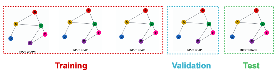
An inductive learning split. Here we would have disparate train, validation and test “graphs”.
In a very layman understanding Transductive datasets shall have only 1 graph but multiple nodes and edges.
Inductive datasets will have multiple graphs with their nodes and edges.
Graph classification would be suitable as an Inductive task, as we want to classifiy unknown new graphs. Detecting a rumour propagation networks is a classification task where we always will have new examples of networks in front of us. Inductive learning tasks aim to generalize to unseen examples.
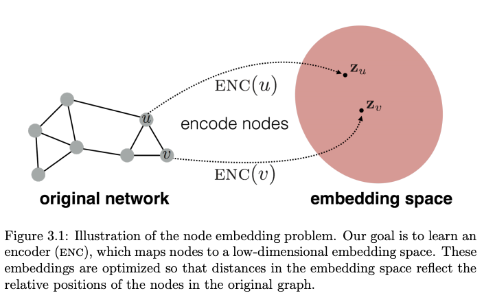
What are Node embeddings?
A graph is defined by its set of nodes and edges. As always, ML models can only interepret a vector or a number.
Node embeddings provide a way to attach meaningful identifying information to nodes. Once we have node level embeddings, we can aggregate these in different ways to achieve a graph level definition. Node embeddings aim to summarize the information of a graph dataset numerically:
1) Structural relation of a node with other nodes in the graph: How is this node positioned in the graph? How central or connected this node is?
2) Feature/information contained in the node itself: Are these nodes describing ages of people , connected together in a friendship network?
Traditionally before graph deep learning methods crept in, node embeddings were developed using manually defined graph properties[3]. It could be the degree of a node. Or more intricate mathemtical properties such as Node centrality or Eigenvector centrality. The choice of picking these properties of nodes while learning the embeddings, would depend on what is the final task you are aiming to train your model for. So it would make a great case to use Node centrality as a useful feature, if the model wants to look at a social network graph and predict celebrities/influencers in a social network.
In order to start with the embeddings training process, the oldest trick in the book is to have a learning objective make sure that your embeds have some actual meaning. For example ensuring that similar nodes in the embedding space have less distance to each other, while dis-similar nodes are far apart. This idea is similar to what we try to do when we learn word ‘embeddings’ in NLP.
Though these days hand crafted features are not favoured. Defining node features manually is laborious and reminiscient of the old days of computer vision defining haar and surf features . Instead now we do graph representation learning directly.
Graph embedding:
Taking everything to embedding space land
We have to be mindful that embedding of a node ‘u’ would be impacted by it’s neighbouring node ‘v’. And this neighbouring node would be impacted by its own neighbours, let’s say,’w’. Hence it would be natural to expect a recursive nature for these node embedding updates.
Some simple ways to embed can be either to encode a node, and then reconstruct the embedding using a decoder. The training loss could measure the pairwise distance, say $ loss(Z_u, Z_v) $, from connected nodes u and v. Ideally neighbouring nodes should have less distance.
Another class of approaches , called factorization based approach, where the task can be seen as using matrix factorization to learn a low-dimensional approximation of a node-node similarity matrix S, where S generalizes the adjacency matrix and captures some userdefined notion of node-node similarity. Their loss functions can be minimized using factorization algorithms, such as the singular value decomposition (SVD). Indeed, by stacking the node embeddings. Factorization based embedding approaches are the ones where random walks are involved and the objective is of the form of a matrix decomposition.
Why is everyone hell bent on achieving the similarity of neighbouring Nodes embedding?
Nodes which have an edge between them, or are neighbours (1-hop, 2-hop, k-hop) would share similar properties. Why? Because most probably graphs try to represent the relations and connection between all the nodes/entities.
For example, if you think of a Football team’s formation as a graph (say 4-4-2), where nodes would be players, player abilities the node features, and relation/chemistry between different players the graph edges. Players connected to each other would most likely be similar players: a defender to defender edge, or midfileder to midfielder egde.
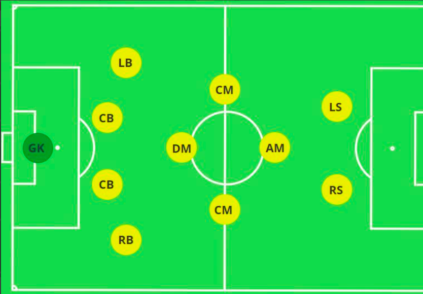
football formation as graphs
The node embeddings is supposed to capture a ‘summary’ of the topology of the graph and node information packaged into a numerical value.
Classical approaches for node embedding
Random walk strategies are often talked about in graph representation learning literature. The intuition behind a random walk strategy goes like this:
“For a node, we want to learn feature representations that are predictive of the nodes in its random walk neighborhood. A random walk neighbourhood being just a set of random paths from a source node to some destination nodes”
If you were to choose a path from one node,’u’, to another on a graph,’v’, and write a probability for the movement between these two nodes:
$ P(v \mid z_u) = {z_u}^{T} {z_v} $
This probability of reaching node v, if starting from node u with embedding z. The more two nodes are connected or are in the neighbourhood, the higher you would have this probability. Ideally using these update rules would also gather other useful implicit information apart from the network topology.
Choosing to use or discard node features can be a training choice. If you are beginning with only the adjacency matrix representation,then you would be lacking in node features. You can either choose to add constant values to all nodes for node features or add unique ids (say 1 hot encoding) to the nodes.
GCN
Before going towards a GCN (Graph Convolution Network), lets check what happens inside a single GNN layer (Graph Neural Network).
The two most important equations are:
$ m_{N(u)} = \sum_{v \in N(u)} h_v $
$ Update (h_u, m_{N(u)}) = \sigma (W_{self}h_u + W_{neighbor}m_{N(u)}) $
where :
$ m_{N(u)} = Aggregate^{(k)} ( {h_v}^{(k)} , \forall v \in N(u)) $
$h_i$ represents node embedding for a node i.
The first equation is called a message passing equation. ‘Sum’ operator is aggregating all the contributing information from the neighbourhood of this node u, $N(u)$. The second equaion represents the update rule for a node embedding $h_u$ after each iteration,’k’. Aggregation involves a combination of $W_{neigh} x $(embedding value of the neighbourhood) and $W_{self} x $ (the node itself). This is often referred to as self updates.
Each node ‘u’ has some relation to its neighbouring node ‘v’, which in turn would be connected to it’s own neighbour node ,let’s say ‘w’. Any expression for node embedding update is bound to be recursive in nature. There is good pictorial description of these updates at this topbots blog. The updates happening are analogous to the “$ product + sum $” approach used in convolution networks, and hence the name. Check the link for more detailed explanation on this aspect.
Notice that the aggregation happens only in the neighborhood and not all across the graph.
Another thing to observe is that the update equation gives scope for manipulation. Having a non linearity $(\sigma)$ with some weight $W$ is one way, but we could also try concatenations. Something like this maybe for a single GNN layer: $ {h_u}^{(k)} = CONCAT (AGG ({m_v}^{(k)} , v \in N(u)) , {m_u}^{(k)}) $
The graph level equation for this would be (careful this is a matrix form now):
$ H^{(k)} = \sigma (A H^{(k-1)} {W_{neigh}}^{(k)} + H^{(k-1)}{W_{self}}^{(k)}) $
where ‘A’ is an Adjacency matrix representing egdes.
The form of this equation kind of looks familiar…cue the formula we have for a MLP. Graph Convolution Networks ultimately are not that different at all then…
A more simplified equation can be achieved if we imagine that there is a shared weight parameter weight , combing both $W_{neigh}$ and $W_{self}$
$ H^{(k)} = \sigma ( (A + I) H^{(k-1)} W^{(k)}) $ Notice the difference between this and the previous graph level equation.
Naturally the aggregation operation opens up the case for use of attention over assigning importance to each of the “message” contributions from different nodes. This shall be expanded on when discussing about ‘Graph Attention Networks’ (GAT).
Question : It is mentioned that stacking L layers of GCN , leads to neighborhood aggregation till L neighbouring nodes. Though honestly this important point is not very clear to me yet.
For a GCN there would be this aggregation along with a normalization constant:
$ {h_u}^{(k+1)} = \sigma ( \sum_{j \in N(u)} \frac{1}{c_{uj}} W^k {h_j}^k ) $
Do you wonder what changed here?
$c_{uj}$ is a normalization constant. Imagine that if a node ‘u’ has 100 nodes in its neighbourhood, and another node ‘v’ with just 2. The message passing contribution would be a large value for the first node u (this will be obvious if your refer back to the aggregation function for each node). While for the node v with a very small neighbourhood, it woud be negligible. Normalization based on penalizing the node degree would be helpful here for training stability. Because otherwise one node would end up with values on a very different scale compared to other nodes, and these node embeddings would not mean anything.
Though this normalization penalty can lead to loss of structural information, as maybe a very high degree node is a high degree node for some reason. So its another training decision to be made. Normalization can be very useful when we are more interested in the node features, than the graph structure information itself.
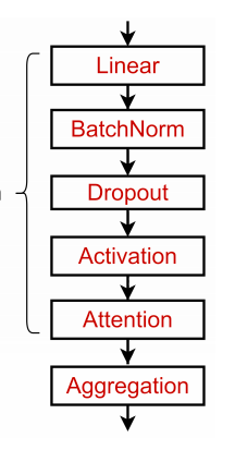
The magic box unravelled. Aggregation is the secret ingredient : A Graph layer stack
By the way GCN can work both with/without node features.
What happens during training ?
From the graph deep learning book written by Hamilton et al [4] : “After the first iteration (k = 1), every node embedding contains information from its 1-hop neighborhood, i.e., every node embedding contains information about the features of its immediate graph neighbors, which can be reached by a path of length 1 in the graph; after the second iteration (k = 2) every node embedding contains information from its 2-hop neighborhood; and in general, after k iterations every node embedding contains information about its k-hop neighborhood”
In a k-layer GNN, each node has a receptive field of k-hop neighborhood. Receptive field is ML terminology for saying what comes under the ‘scope/purview’ of an operation.
Adding too many GNN layers can lead to a scenario where all nodes end up with the same value of embeddings , called ‘over smoothing’. Why does over smoothing happen? Imagine that if every node was in the scope of every other node, it means that they all impact each other. Hence all nodes end up in same receptive fields, with same final aggregated values.
Adding MLP layers or skip connections in between GNN layers can be a way to avoid this problem. MLP layers would help learn some better combination methods, and skip connections would help preserve useful information between far apart layers.
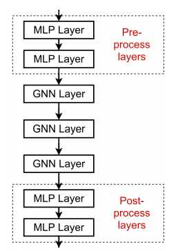
Magic box unravelled again: gnn with mlp
GAT
GAT (Graph attention networks) give weights to messages passed from each node according to its importance. The connection weights learn how to value each of these messages during model training. In this scenario each node in the neighbourhood would not be contributing equally.
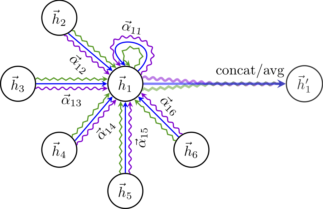
Graph attention network. image from Veličković et al. Notice the three coloured lines on each edge, representing 3 attention heads values in the original paper
For a graph attention network:
$ {h_u}^{(k+1)} = \sigma ( \sum_{j \in N(u)} {\alpha_{uj}}^l {z_j}^k )$
Update equation for a node u, with embedding $h_u$, where its neighbourhood $N(u)$ has its contributions weighted by $\alpha_{uj}$. $\alpha_{uj}$ can be thought of as capturing the edge importane.
GraphSage Network
Remember when we wrote the aggregator function in the message passing equation earlier?
Graph sage aims to train aggregator functions, instead of obsessing about embeddings of nodes. In layman terms this means, that it has developed a knowledge of how to best utilize the neighbourhood $N(u)$ rather than being finetuned to the specifics of node ‘u’ itself. Hence Graph sage can be termed as capable of doing ‘inductive’ network by definiton. Graph sage can use node features (say text or image information).
Graph Sage network uses a non linearity and aggregation on top of the original aggregation:
This is the two stage aggregation: $ {h_u}^{(k)} = \sigma ( W^{(k)}). CONCAT ({h_u}^{(k-1)} , (AGG ({h_v}^{(k-1)} , u \in N(u)))) $
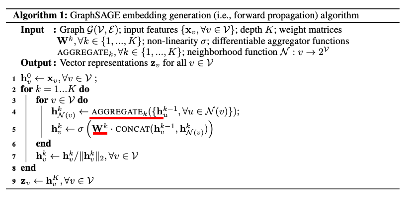
graphSage algorithm, trainable aggregator in red

graph sage loss
The loss objective of GraphSage makes use of Negative Sampling. Negative sampling basically comes to our rescue whenever we end up in a situation where we need to have the whole set of samples of our training but we choose to just ‘sample’ some data points at random, knowing that these random samples would be a ‘negative target’ with high probabilty
From the paper “v is a node that co-occurs near u on fixed-length random walk, $\sigma$ is the sigmoid function, $P_n$ is a negative sampling distribution, and Q defines the number of negative samples. Importantly, unlike previous embedding approaches, the representations zu that we feed into this loss function are generated from the features contained within a node’s local neighborhood, rather than training a unique embedding for each node (via an embedding look-up)”
Wait .. SO how do predictions even work here?
Now that we have our mishmash of node embeddings ready with us, how do we put these node embeddings to use for a simple classification task?
If we have d dimensional emebddings ,for a node v, with some lable $y_v$.
1)For a node level prediction, we can apply a prediction layer on top of the node embeddings:
$ \hat{y_v} = W_{predict} ( {h_v}^{(k)} \in {R}^d ) $
2) For edge level prediction, we can use a pair of node embeddings:
$ \hat{y_{uv}} = W_{predict} ( {h_v}^{(k)},{h_u}^{(k)} ) $
You can do either concat or dot of the two node embeddings for the pair combination/aggreation.
3) For graph level prediction, we would want to use embedding of all the nodes:
$ \hat{y_g} = Prediction layer ( {h_v}^{(k)} \in {R}^d , \forall v \in G ) $
We can combine/pool all these node embeddings based on our problem, using either Max, Mean or Sum combination/pooling. We can also try developing a hierarchial pooling method, if we don’t want to loose useful information in the process of pooling nodes trivially.
Today’s example project
Nature of fake information
Fake information can be spread out by a network of colluders, who aim to actively get a ‘rumour’popular enough to be viral, by first sharing it in their own networks.
The Fake information in question could be fake images for alleged crimes, politically motivated statements, rumour mongering for sensational gossips or fake news to spread panic. Moderating such content is not always possible due to huge size of modern social platforms where such information is usually spread. Instead of looking at the shared content in isolation, it would be easier to spot a network of such people, colluding together in rumour propagation.
What is this dataset?
Imagine that when a network of people collude together to spread fake news, it would appear as if there are 1) nodes (with the fake news as the node feature) 2) and the connections/retweets/reshares as the graph edges.
UPFD is a dataset of such graphs, where we have both fake news propagation networks, and genuine news networks, extracted from Twitter.
For a single graph, the root node represents the source news, and leaf nodes represent Twitter users who retweeted the same root news. A user node has an edge to the news node if and only if the user retweeted the root news directly. Two user nodes have an edge if and only if one user retweeted the root news from the other user. Four different node features are encoded using different encoders.
This dataset is scraped from Politifact.com, which lists many news snippets and then comments if they are True or False, which can act as label for the source information.
Ending notes
The data had choice of using Bert features (768 dim) or simple user profile information (10 dim). I used the Bert text representations of the fake information text. Upon running each of the three models, and checking the test accuracies , there did not seem to be a big difference between the three.
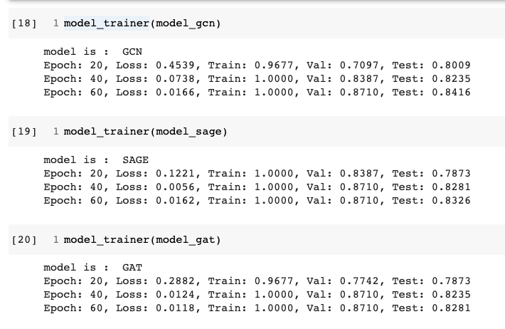
All three models seem to have achieved smilar final test accuracies
Possible explanation for this situation could be that the graph dataset in question is simple enough and does not need a lot of model capacity. Honestly I don’t know :) Maybe this is a question for further investigation.
References
- User Preference-aware Fake News Detection, Dou et al
- Automatically Identifying Fake News in Popular Twitter Threads, Buntain et al
- Stanford course slides Jure leskovec
- William Hamilton Graph Representation Learning book
- Guiseppe Futia, Understanding Building blocks of Graph neural networks
- Guiseppe Futia, Graph Attention Networks under the hood
- Inductive Representation Learning on Large Graphs Hamilton et al
- Kipf graph convolution networks
- Topbots blog on GCN